Deep Dive into EchoCLIP – Pass The Torch

Introduction

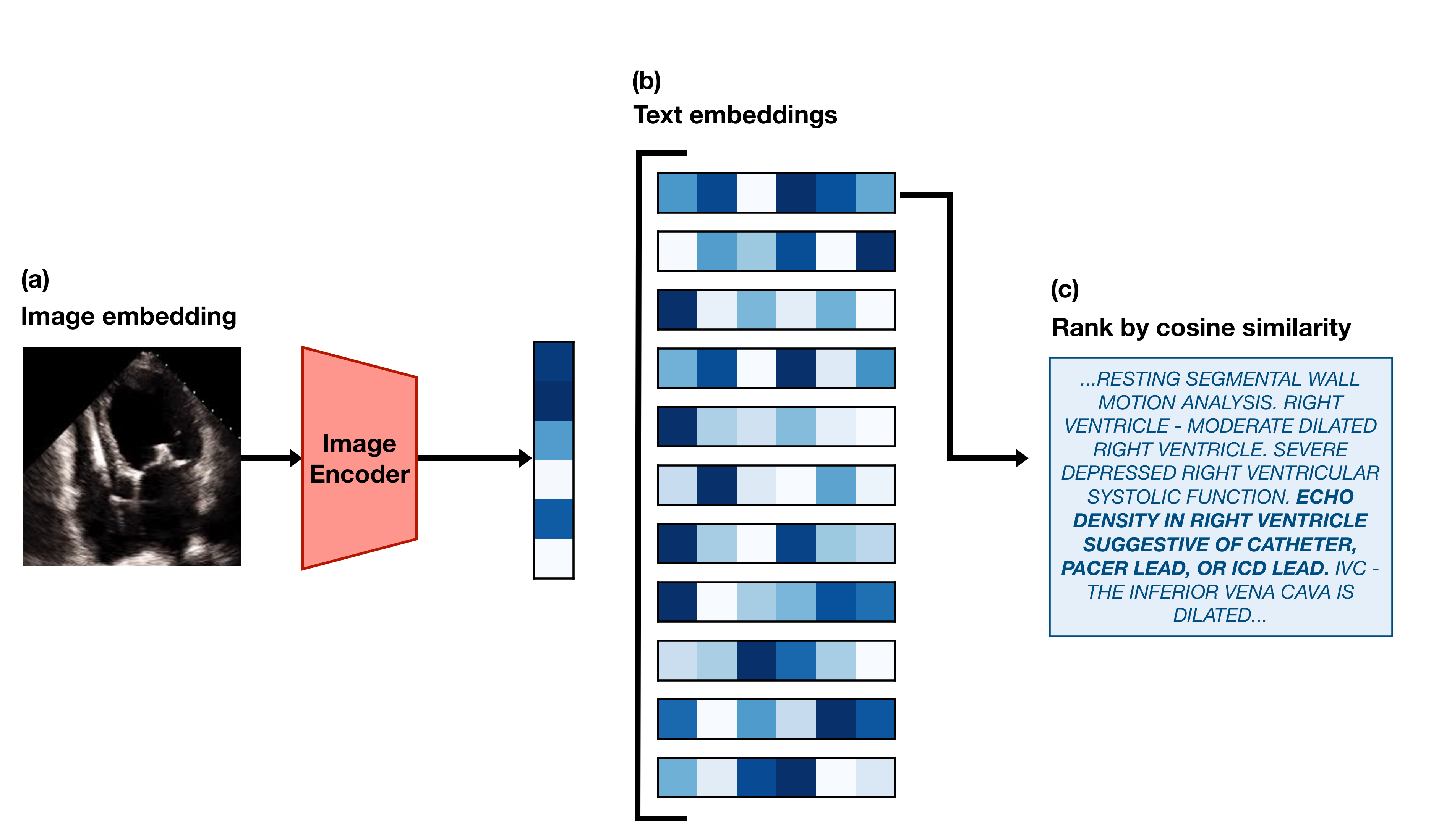
This post is a code-forward deep dive into EchoCLIP, a vision-language model for echocardiogram interpretation. The code repository for EchoCLIP is available on GitHub and the accompanying Nature paper is available at https://www.nature.com/articles/s41591-024-02959-y#Sec9.

TODO: Add more details about EchoCLIP, its relation to CLIP

Initialization of EchoCLIP

echo_clip, _, preprocess_val = create_model_and_transforms(
    "hf-hub:mkaichristensen/echo-clip", precision="fp32", device="cpu"
)

create_model_and_transforms() is a function from the open_clip library that loads a pretrained CLIP model from Hugging Face Hub, hf-hub:mkaichristensen/echo-clip, sets it to 32-bit precision, and runs it on a CPU.

Video Embedding

test_video = read_avi(
    "example_video.avi",
    (224, 224),
)
test_video = torch.stack(
    [preprocess_val(T.ToPILImage()(frame)) for frame in test_video], dim=0
)
test_video = test_video[0:min(40, len(test_video)):2]

The code above reads an example echocardiogram video, preprocesses each frame using the validation transformations defined in preprocess_val, and selects every other frame up to a maximum of 40 frames. The resulting test_video tensor has shape (num_frames, 3, 224, 224).

test_video_embedding = F.normalize(echo_clip.encode_image(test_video), dim=-1)

Normalizes the CLIP embedding for easier calculation of cosine similarity later on.

Cosine similarity = (A . B) / (||A|| * ||B||) and when A and B are normalized to unit length, this simplifies to A . B, which is just the dot product of the two vectors. Much cheaper than calculating the full cosine similarity with unnormalized vectors.

In this case, A would be the test video embedding and B would be the prompt embedding.

Text Embedding

pacemaker_prompts = tokenize(pacemaker_prompts).cpu()

Use the CLIP BPE tokenizer to tokenize the pacemaker prompts

['ECHO DENSITY IN RIGHT VENTRICLE SUGGESTIVE OF CATHETER, PACER LEAD, OR ICD LEAD. ',
 'ECHO DENSITY IN RIGHT ATRIUM SUGGESTIVE OF CATHETER, PACER LEAD, OR ICD LEAD. ']

and the move the tokenized prompts to the CPU for later use in calculating similarity with the video embedding.

pacemaker_prompt_embeddings = F.normalize(
    echo_clip.encode_text(pacemaker_prompts), dim=-1
)

Encode the tokenized pacemaker prompts using the CLIP text encoder and normalize the resulting embeddings for later use in calculating cosine similarity with the video embedding.

pacemaker_predictions = compute_binary_metric(
    test_video_embedding, pacemaker_prompt_embeddings
)

def compute_binary_metric(
    video_embeddings: torch.Tensor,
    prompt_embeddings: torch.Tensor,
):
    per_frame_similarities = video_embeddings @ prompt_embeddings.T
    # Average along the candidate dimension and frame dimension
    predictions = per_frame_similarities.mean(dim=-1).mean(dim=-1)

    return predictions

The compute_binary_metric function calculates the cosine similarity between the video embeddings and the prompt embeddings by performing a matrix multiplication (dot product) between the video embeddings and the transposed prompt embeddings. This results in a tensor of shape (batch_size, num_frames, num_prompts). The function then averages the similarities across both the candidate dimension (e.g., if there are 2 pacemaker prompts, their similarities are averaged into one score per frame) and the frame dimension (collapses all frame-level scores into one score per video) to produce a single prediction score for each video in the batch.

Predicting Continuous Values

ejection_fraction_prompts = zero_shot_prompts["ejection_fraction"]

['THE LEFT VENTRICULAR EJECTION FRACTION IS ESTIMATED TO BE <#>% ',
 'LV EJECTION FRACTION IS <#>%. ']

Ejection fraction can range from 0% to 100%, so we make 100 versions of each prompt, replacing <#> with each integer from 0 to 100.

ejection_fraction_prompts = tokenize(ejection_fraction_prompts).cpu()
ejection_fraction_embeddings = F.normalize(
    echo_clip.encode_text(ejection_fraction_prompts), dim=-1
)

Once again tokenize and embed the ejection fraction prompts using the CLIP text encoder, and normalize the resulting embeddings for later use in calculating cosine similarity with the video embedding.

ejection_fraction_predictions = compute_regression_metric(
    test_video_embedding, ejection_fraction_embeddings, prompt_values
)

Computing the regression metric:

def compute_regression_metric(
    video_embeddings: torch.Tensor,
    prompt_embeddings: torch.Tensor,
    prompt_values: torch.Tensor,
):
    per_frame_similarities = (
        video_embeddings @ prompt_embeddings.T
    )  # (N x Frames x Candidates)

    # Sort the candidates by their similarity to the video
    ranked_candidate_phrase_indices = torch.argsort(
        per_frame_similarities, dim=-1, descending=True
    )

    # Convert matrix of indices to their corresponding continuous values.
    prompt_values = torch.tensor(
        prompt_values, device=video_embeddings.device
    )  # (N x Frames x Candidates)
    all_frames_ranked_values = prompt_values[ranked_candidate_phrase_indices]

    # Taking the mean along dim=1 collapses the frames dimension
    avg_frame_ranked_values = all_frames_ranked_values.float().mean(
        dim=1
    )  # (N x Candidates)

    # The median of only the top 20% of predicted values is taken
    # as the final predicted value
    twenty_percent = int(avg_frame_ranked_values.shape[1] * 0.2)
    final_prediction = avg_frame_ranked_values[:, :twenty_percent].median(dim=-1)[0]

    return final_prediction

Conclusion

In this post, we walked through the EchoPrime codebase — from model initialization with pre-trained weights, to how the demo notebook leverages similarity to historical echo studies to predict cardiac phenotypes and generate structured reports.